Summary

This study in this theme is aimed to understand the regional circulation pattern in the East Indian Ocean, from the Indonesian Throughflow to the Leeuwin Current, their annual, interannual, decadal variability, and the climate change impact. The Throughflow-Leeuwin Current system is not only important for regional climate, such as Perth rainfall, it is also a key environment factor for WA fisheries and coastal ecosystem.

Here we highlight some recent progress from the SRFME climate research on these topics. We first introduce the regional circulation patterns in the East Indian Ocean, and the annual climatology of the Leeuwin Current. Then we discuss the two major internanuual variation modes in the Pacific and Indian Ocean. The ENSO signal originated from the Pacific has great impact on the regional circulation. The independent mode in the Indian Ocean, the Indian Ocean Dipole, also can affect regional water mass balance.

Future study within this theme will probe into long-term variability, like the decadal oscillation, and climate change. SRFME has funded a collaborative project between CSIRO Marine Research, University of Western Australia, and CSIRO Mathematics and Information Sciences to research these issues.

Regional Circulation in the East Indian Ocean

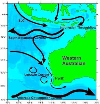The dominant ocean surface current in the southeast Indian Ocean off the Western Australian coast is the south-flowing Leeuwin Current. The Indonesian Throughflow transports warm, low-density tropical Pacific water into the East Indian Ocean through the Indonesian Archipelagos, setting up an anomalous strong north-south pressure gradient. The pressure gradient overcomes the northward local wind stress, and drives an eastward onshore flow that feeds the Leeuwin Current. Part of the Throughflow water joins the westward flowing South Equatorial Current, and part directly flows into the Leeuwin Current. The semi-annual South Java Current (SJC) may also affect the water mass balance in this region. The impact of the Antarctic Circumpolar Current on the Leeuwin Current is still little unknown.

There is also meso-scale variability that related to these large-scale circulation structure. Such as the South Equatorial Current can become unstable and meanders during the second half of the year when the current is intensified. The Leeuwin Current is also meandering and eddy-shedding. The interannual variations of both the large-scale circulation structure and the meso-scale eddy in this region are strongly affected by signals from the Pacific ENSO signals and the tropical Indian Ocean.

Annual Cycle of the Leeuwin Current Climatology off Perth

Before we discuss the annual cycle of the Leeuwin Current climatology, we first looked at the local air-sea forcings in this region. This air-sea flux product is taken at a grid point close to Perth from the Southampton Oceanography Centre.

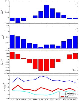
There are clear annual cycles in both the eastward and northward wind stress components off Perth. The annual mean zonal and meridional wind stresses are 0.02 and 0.06 N m^-2 respectively. The eastward wind stress is strong during austral winter, bringing warm moist air inland to cause winter rainfall around Perth. The peak eastward wind stress of 0.11 N m^-2 occurs in July. The wind is weakly westward during October to March. The meridional component of the wind is always northward, stronger during austral summer and with peak wind stress of 0.12 N m^-2 in January.

Typical of mid-latitude, a strong annual cycle of net air-sea heat flux is found off Perth. The ocean receives heat during summer (November to March), but has a stronger heat loss during winter. The peak heat loss is more than 200 Wm^-2 in June-July, and the annual mean heat loss is 37 Wm^-2. Evaporation is stronger than precipitation all year round. Both the precipitation and evaporation rates peak during winter season, and the net freshwater loss is around 2-4 mm day^-1 and has only a weak annual cycle.

Fremantle sea level has been used as an index for the Leeuwin Current strength in fisheries studies during the past decade, because of lacking long-term monitoring of the Leeuwin Current. How these two variables are linked together is a research topic of this SRFME theme, and here we first look at their annual cycles.

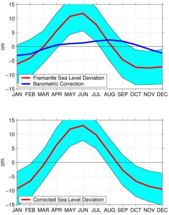
An inverted barometric correction is necessary to use the sea level data for ocean dynamics research. We use NCEP sea surface atmospheric pressure for this correction, that is, with every 1 mb increase of air pressure, the sea level is increased by 1 cm.

The inverted barometric correction increases the Fremantle sea level annual variation range but reduces its interannual variability. Before correction, the Fremantle sea level deviation has an annual variation range of about 19 cm and reaches its peak value during June. The sea level atmospheric pressure has an annual range of about 6 cm and is highest during the late winter of July-September. After the inverted barometric correction, the annual range of sea level variation increases to 23 cm, still peaking in June. That is, the atmospheric correction increases the annual range of sea level deviation by about 20%. Also note that the sea level standard deviations after the inverted barometric correction are smaller than those before the correction during most months. This is due to the inversed relationship between the atmospheric pressure in Fremantle and the SOI on the interannual time scale.

Mapping the upper ocean temperature climatology: The upper ocean temperature climatology is determined from the expendable bathy-thermograph (XBT), Conductivity-Temperature-Depth (CTD) and bottle temperature measurement.

Since early 20^th century, large number of observations from commercial ships, scientific research vessels, fisheries, and Australian Navy have been collected offshore of Western Australia. The small inset shows an example of data distribution off Perth. The data distribution is irregular in time and space. To construct the climatology on regular time and space grid needs both statistics and art. We use a method called LOESS (Locally Weighted Least Square) to map the temperature data, that is, we select observation data within a certain radius to fit with a smooth structure. The grey dots in the inset show the positions of the XBT/CTD observations, which are mapped onto the solids dots, the grid points that the temperature climatology. A searching radius in both space and time is determined for each grid point as shown. Then the data within the searching ellipse is fitted with

.

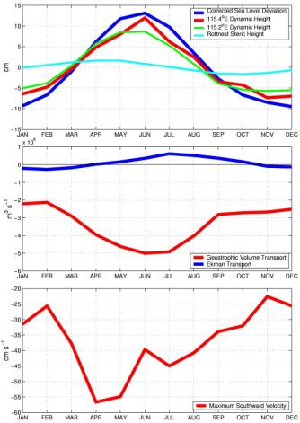
With the temperature climatology and inferred salinity data, we can derive the ocean density and then the pressure field. From the water density, we use a Geostrophic relation to derive the ocean current, that is, we assume the pressure gradient is totally balanced the earth rotation forcing. The geostrophic balance of the Leeuwin Current can be expressed as . Here f=-7.7´10^-5 s^-1 is the Coriolis parameter, twice of the earth rotation rate, at 32°S, v is meridional velocity, r₀=1025 kg m^-3 is the mean density, and p is the pressure perturbation. At sea surface, the pressure is calculated as p=r₀gV, where g is the gravity constant and V is the sea surface elevation. At the eastern most grid point, the sea surface height variation from the temperature climatology is closely followed by the Fremantle sea level, which means that on the annual time scale, Fremantle sea level is determined by the Leeuwin Current pressure forcing. The local heat expansion (Rosttnest steric height) only has minor effect.

Maximum southward velocity peaks in April in the Leeuwin Current along 32°S, while the integrated southward velocity, the Leeuwin Current volume transport peaks in June. The annual mean Leeuwin Current volume transport is 3.4 Sv (10⁶ m³s^-1). Local wind driven transport (Ekman transport) is rather weak.

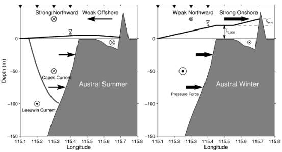A sketch is used to show the annual cycle of pressure and local wind forcing on the Fremantle sea level variation. During the austral summer, the Leeuwin Current is weak and the pressure gradient across the current is also weak. Thus, the pressure force exerted on the continental shelf from the Leeuwin Current is weak and the Fremantle sea level is lower. The offshore zonal wind may contribute to further lower the Fremantle sea level. During austral winter, the Leeuwin Current is stronger and the pressure gradient across the current is stronger. This raises the baroclinic component of the pressure forcing exerted on the continental shelf and the Fremantle sea level. The onshore wind during the winter season also contributes to further raise the sea level at Fremantle.

ENSO Influences on the Leeuwin Current

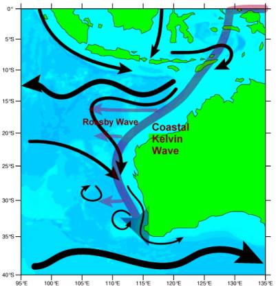The annual and interannual variations in the tropical western Pacific propagate poleward along the northwest to west coast of Australia as shown by the light blue colours in the sketch. This signal can be observed from the coastal tide gauge measurements, as well long term upper ocean thermal data observed by XBT (Feng et al., 2003). Along the poleward propagation, the coastal signal can also propagate westward as Rossby wave, which translate the coastal sea level into the ocean interior. Both the coastal Kelvin wave and the westward Rossby wave have significant impacts on the regional circulation pattern. Such as, during an El Niño year, both the Indonesian Throughflow and the Leeuwin Current becomes weaker, and it is on the contrary during a La Niña year. A list of El Niño and La Niña years during 1950-2000 in the below table are determined from the annual mean Southern Oscillation index (SOI), which is the sea level atmospheric pressure difference between Tahiti and Dalwin. SOI is an important index for the El Niño and La Niña events. The real time SOI index can be obtained from the Bureau of Meteorology website.

El Niño Years	1953, 1965, 1972, 1977, 1982, 1987, 1991, 1992, 1993, 1994, 1997
La Niña Years	1950, 1955, 1956, 1971, 1973, 1974, 1975, 1988, 1989, 1996,1999, 2000

On the right, we show a short time series of upper ocean temperature data at the southern end of a repeated XBT section at 31.43°S, 114.7°E off Perth. This is taken from an optimal interpolated product along a commercial ship line from Fremantle to Singapore.

There are 5 El Niño Years and 4 La Niña Year during the time period from 1988 to 2000 (Table). Qualitatively, the sea surface temperature is slightly higher and the surface mixed layer and thermocline depths are deeper during the La Niña years, while the opposites occur during the El Niño years. The surface dynamic height is the surface pressure anomaly relative to a reference depth, 300m.

A detailed comparison between dynamic height at the location and the Fremantle sea level is rather consistent. The dynamic height tends to lead the Fremantle sea level by one month or so during most years. This delayed relationship may be a manifest of the retardation effect due to bottom friction on the continental shelf, like the case in an “ENSO jet”.

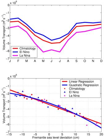
Temperature scenarios during El Niño and La Niña are also derived from the temperature climatology. During the La Niña years, the Leeuwin Current is strong, and it is weak during the El Niño years. The annual cycle of the Leeuwin Current transport during the ENSO scenarios are similar to the climatology.

The regression between the volume transport and Fremantle sea level deviation is calculated by treating the monthly value during different scenarios as individual data input, and fitting with a linear function or a quadratic function. Results show that the linear function is good enough to describe the relationship between the volume transport and the sea level deviation, due to the small variation range of the sea level deviation. There is a 0.13 Sv change of volume transport by every 1 cm of sea level deviation.

In conclusion, the dominant annual and interannual Fremantle sea level variations are associated with the baroclinic pressure forcing of the Leeuwin Current, which justifies the use of Fremantle sea level as an index for the Leeuwin Current strength on the annual and interannual time scales. The Leeuwin Current volume transport has a quasi-linear relationship with the Fremantle sea level deviation.

Subsurface Evolution of the Indian Ocean Dipole

An Indian Ocean Dipole event, also so-called Indian Ocean “ENSO”, is characterized with anomalous higher than normal sea surface temperature (SST) in the tropical western Indian Ocean, and lower than normal SST in the tropical eastern Indian Ocean, as well as reversed, anomalous westward wind on the equator.

An Indian Ocean Dipole event starts with anomalous SST cooling along the Sumatra-Java coast in the eastern Indian Ocean during May-June. The normal equatorial westerly winds during June-August weaken and reverse direction. And an Indian Ocean Dipole event peaks near September-October, with warmer than usual SST over large parts of the western basin.

The figure shows the SST anomaly (in colour) and the wind anomaly (in arrows) during the initial and peak phases of a dipole event.

From the expendable bathy-thermograph (XBT) temperature data near the Sumatra-Java coast, an Indian Ocean Dipole event is initiated by an anomalous upwelling along the Sumatra-Java coast at the start of the normal upwelling season in May-June. This enhances cooling of sea surface temperature (SST) in the eastern Indian Ocean, which couples with a westward wind anomaly along the equator and drives rapid growth of Indian Ocean Dipole.

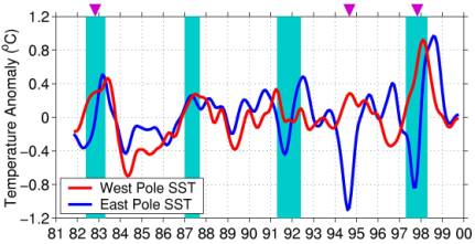
1994 and 1997 are two dipole event years during the last decade. The strong upwellings are seen in the temperature time series, and the anomaly field.

From extended empirical orthogonal function (EEOF) analysis of the satellite sea level anomaly, the wind anomaly and associated Ekman pumping generate off-equatorial Rossby waves that travel westward, deepen the thermocline and warm SST in the western Indian Ocean, causing the peak of an Indian Ocean Dipole event a few months after it begins. The decay of an Indian Ocean Dipole event is characterized by a slow eastward propagation of warm anomaly along the equator.

The deepened thermocline arrives at the eastern boundary and reduces the rate of cooling during the next upwelling season. This causes a positive SST anomaly in the eastern Indian Ocean in the following year of an Indian Ocean Dipole event. The evolution of the event during two upwelling seasons involves the SST, wind, and subsurface temperature. Thus, we say that the Indian Ocean dipole tends to have a two-year time scale. In the below figure, the dipoles years are shown with inverted arrows and the two-year time scale of the SST evolution is clearly seen.

The observed behaviour of the tropical Indian Ocean and the role of internal ocean dynamics suggest a coupled ocean/atmosphere instability that may be initiated by ENSO or other anomalies during the early Sumatra-Java upwelling season; however, proof of its existence will require further research, including modelling and model validation with these observations.

References:

Feng, M., G. Meyers, and S. Wijffels, 2001: Interannual upper ocean variability in the tropical Indian Ocean. Geophysical Research Letters, 28, 4151-5154.

Feng, M., and S. Wijffels, 2002: Intraseasonal variability in the South Equatorial Current of the East Indian Ocean. Journal of Physical Oceanography, 32, 265-277.

Feng, M., and G. Meyers, 2002: Interannual variability in the tropical Indian Ocean: a two-year time scale of the Indian Ocean dipole. Deep-Sea Research, in press.

Feng, M., G. Meyers, A. Pearce, and S. Wijffels, On the relationship between the annual/interannual variations of Fremantle sea level and the Leeuwin Current. Submitted.

This page was maintained by Ming Feng and was last updated 6 February 2003.